Think of an event.

The event could be anything, whether desirable or undesirable. An A&E arrival, an earthquake, a handbag sale, a property viewing, a virus infection, a death.

When did that event last happen? And is the time since that event happened typical, predictable or exceptional?

Asking these questions can yield deep insights about a system and its processes. The elapsed time between two events is a property of a system which is often invisible.

We sometimes use inter-event timing when talking about Mean Time Between Failures (MTBF) in engineering or cycle & lead times in manufacturing.

The concept of recency goes beyond this and arises in many, many systems. It is fundamental to understanding flow and variability of work and seeking ‘profound knowledge’ as W. Edwards Deming might say.

It is easy to think of the rate of events within some time period eg. orders per month, appointments each week as having similar value. But counts of things over some time period are aggregated measures of throughput which serve a different purpose.

Taking a rate such as 10 transactions over a minute and inverting with 1/rate we get a frequency of 1 transaction every 6 seconds. But this time is a mean average with an implicitly smooth inter-arrival time. What if those transactions all happened in the first 20 seconds, followed by 40 seconds of nothing?

Recency is a measurement which reveals this insight; the variability of the time between events, the essence of flow. We can use it to see short term bursts or droughts of work and whether or not these are predictable.

Why does this matter?

Many processes form a network of queues with a long run behaviour governed by Little’s Law. When capacity is occupied by work in a process, new work has to wait in a backlog to be serviced. Transient bursts of work may consume capacity quickly, forcing new work to wait longer. This converts a variation in arrival rate into a variation in queuing delay. These delay spikes may now produce an inconsistent user experience which is far from an expected distribution.

Flow systems may deal with this unpredictability using a pull model, admitting work at a constant rate, a ‘Takt Time’. With perfect flow, work is pipelined without waiting anywhere, moving through a process without ‘touching the sides’. The amount of work in each part of the process never exceeds some manageable ‘WIP’ limit, allowing capacity to be optimised, balanced to act on the work.

Recency isn’t a commonly used or accessible term. Expressing the measure as an ‘inter-event time’, ‘time between events’ is more descriptive. The words ‘cadence’, ‘beat’, ‘pulse’ or ‘rhythm’ might be more suitable in some settings.

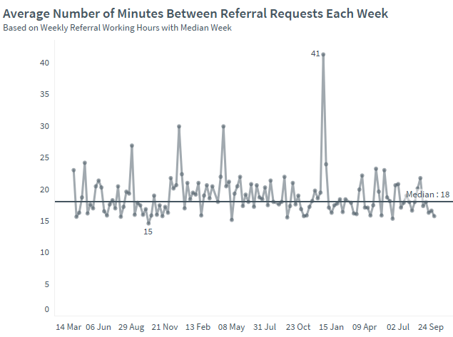
Perhaps just as important is the interpretation of these inter-event timings. By far the most powerful method is visualisation in a line chart, preferably with statistical control lines. An XmR chart is the ‘swiss army knife’ choice but a Mean or median X-bar chart works too.

Each event is a discrete category on the X-axis, as a sequentially numbered item or, more usefully a date. The elapsed time in suitable units between each event and the next one is then plotted on the Y-axis, joined by a line. Here, unless there’s a difference between the date/time stamps for each event, the recency Y-value will be zero. A central line and upper/lower process limits are then computed for the Y-values.

There will be natural gaps in the recency of work such as overnight and weekends which might lead us to mask out non-working time from this chart. High volumes of events can be more difficult to plot too.

Through the lens of recency, we can see why batches are the enemy of flow. A batch produces work items which are spaced at shorter intervals, followed by a longer interval until the next batch. Revealed through an XmR chart, the process behaviour can flap alarmingly out of statistical control. Its easy to see why absorbing and handling this pumping demand in a predictable way is so challenging.

A really useful technique is to use XmR charts look at recency in different parts of a process such as a customer journey. At any process steps where the recency and its variability are shifted, queues will form, however transient. Bottlenecks will be immediately visible, much like a backlog on a Kanban board. Jump plots are another way of revealing this in a visual way. Comparing histograms can be instructive too, revealing different pulse ‘modes’.

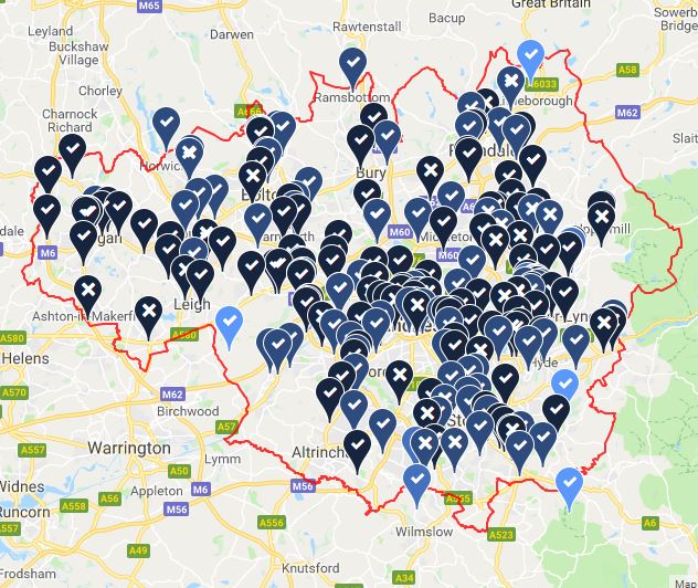
Example – Health

A health provider had an overall referral recency of one every 18 minutes. Stratifying this recency was revealing both in terms of which service had the most arrival intensity but also variability. This brought focus to how often a person needed to be triaged by each service as well as thinking about ways of smoothing demand. Holding more frequent admissions team meetings was one option, another was to ‘pull’ a pulse of referral demand every day from the most predictable source.

 

 

 

 

 

 

 

 

 

 

 

Example – Property

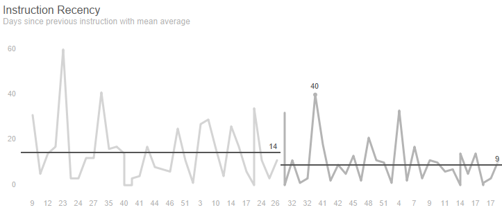
An estate agency had appointed a new branch manager and wanted to understand whether the branch was now winning more property listings and market share. The number of days since the previous instruction was used to detect a positive shift from an instruction every 14 days to one every 9 days.

 

Consider the gender composition of the Board of Directors at 5 companies.

Which company was the least fair when it appointed its 8 board members?

 

 

 

 

 

 

This question echoes familiar claims about the gender balance of leadership teams in companies. Diversity of other forms too.

What does this information tell us about the fairness of each company in making board appointments?

Absolutely nothing.

In fact all 5 companies are fictitious and the board gender composition was generated randomly using coin flips. Every single one of these gender compositions can occur randomly without any causal explanation.

This seems surprising, dissonant. Our brains want to construct plausible stories about possible factors; hiring biases, social responsibility, diversity policies, sector culture etc.

We may still attempt to score, rank, benchmark the diversity of companies using this type of information.

True, the chance of 8 board members of the same sex is far less likely than an even gender split. This is the binomial distribution at work.

This is what statistics is good at: aggregation, summarisation. Statistics can show how gender distribution on boards departs from expected proportions across lots of companies. It can detect true, and unacceptable discrimination at scale. It also helps us to claim with some confidence that groups with shared characteristics are different to others – fashion compared with construction for example – and how that might mirror historic or current social norms.

But we can’t look at the gender of board members at an individual company and make a reliable judgement about whether they were appointed with a gender bias or not. Comparing an individual company to an industry average of some sort isn’t meaningful either. A single-sex 8 person board can occur as a chance outlier rather than by discrimination.

If all our 5 companies truly have a random gender mix, what could they have done differently? Might we actually make a false accusation of bias? Should they have engineered a ‘representative’ gender mix? Or would intervening in a random distribution actually lead to more unfairness?

That’s a dilemma.

One example is how the investment industry compares companies according to their Environmental, Social & Governance (ESG) performance. Some ‘rating’ schemes attempt to score an individual company’s social responsibility based simplistically on the board gender mix. More of one gender = less representative of the population = less socially responsible. Seriously?

At the very least we might try to express the probability of gender bias in an individual company, given base rates (eg. for an occupation, sector) and a binomial expectation. Perhaps thats just not headline-grabbing enough? Do we just want simple claims – such as a gender pay gaps – which confirm our beliefs about unfairness without detecting real, wrongful discrimination?

What does that say about our intuitions when wrestling with the concept of diversity of all forms? Could championing ‘diversity’ as a vague and simplistic ideal even obscure its specific purpose, intent, goals? If we focus on what we can easily see and count, we might fail to seek those true causal factors which make the world a better place.

Here’s an example of a Decision Gallery based on public data from Clean Air Greater Manchester.

The existing data is organised around individual monitoring station locations. This makes it hard to see the big picture of whether air quality is really changing or not. The interpretation is also focused on the achievement of Air Quality Targets (less than 40μg/m3) rather than the big patterns of change.

Our series of 6 Insight Canvases explores the historical Diffusion Tube monitoring station data. It tells a richer story about how Air Quality is changing over time across the Greater Manchester Combined Authorities.

There are two broad questions:

1. Is Air Quality getting better or worse?
2. Where should interventions be focused to make it better?

You can download the Decision Gallery PDFs here

These are designed to be printed on A1-sized panels for a physical gallery but could also be adapted for online content.

With major Congestion Deal and Clean Air Plan initiatives launching in the region, a Decision Gallery is a way to reveal the evidence of whether change is working.

Many more data sources could  be explored by this Decision Gallery, including active monitoring NO2/PM stations, traffic flows & vehicle emissions, population proximity, and health service demands.

A Causal Canvas would also explore the claimed links between congestion, air quality and pollution-related deaths.

We learn by seeking causal explanations for things. If we can reliably attribute effects to causes we can learn how to get more positive effects and fewer negative ones.

But what if we’re not as good at causal attribution as we might hope? See more